library(sf)
library(dplyr)
library(ggplot2)Do-It-Yourself
import pandas as pd
import geopandas as gpd
import contextily as cx
import matplotlib.pyplot as plt
Task I: Photographs in Tokyo
In this task, you will explore patterns in the distribution of the location of photos. We are going to dip our toes in the lake of point data by looking at a sample of geo-referenced photographs in Tokyo. The dataset comes from the GDS Python Book and contains 10,000 photographs voluntarily uploaded to the Flickr service.
Note
We read both files below straight from GitHub, so there is nothing to download — but you do need an internet connection when you run these cells.
Photos
# Read the CSV file into a data frame
tokyo <- read.csv("https://raw.githubusercontent.com/gdsbook/book/master/data/tokyo/tokyo_clean.csv")

head(tokyo)
user_id longitude latitude date_taken
1 10727420@N00 139.7005 35.67400 2010-04-09 17:26:25.0
2 8819274@N04 139.7665 35.70909 2007-02-10 16:08:40.0
3 62068690@N00 139.7656 35.69448 2008-12-21 15:45:31.0
4 49503094041@N01 139.7844 35.54859 2011-11-11 05:48:54.0
5 40443199@N00 139.7688 35.67152 2006-04-06 16:42:49.0
6 52465044@N00 139.6474 35.54845 2009-01-20 20:33:36.0
photo.video_page_url x y
1 http://www.flickr.com/photos/10727420@N00/4545144774/ 15551388 4255856
2 http://www.flickr.com/photos/8819274@N04/2650331694/ 15558738 4260667
3 http://www.flickr.com/photos/62068690@N00/3125862684/ 15558639 4258664
4 http://www.flickr.com/photos/49503094041@N01/6332937940/ 15560727 4238684
5 http://www.flickr.com/photos/40443199@N00/2482548783/ 15558986 4255517
6 http://www.flickr.com/photos/52465044@N00/3222494692/ 15545476 4238666# Read the CSV file into a data frame
tokyo = pd.read_csv("https://raw.githubusercontent.com/gdsbook/book/master/data/tokyo/tokyo_clean.csv")
tokyo.info()<class 'pandas.core.frame.DataFrame'>
RangeIndex: 10000 entries, 0 to 9999
Data columns (total 7 columns):
# Column Non-Null Count Dtype
--- ------ -------------- -----
0 user_id 10000 non-null object
1 longitude 10000 non-null float64
2 latitude 10000 non-null float64
3 date_taken 10000 non-null object
4 photo/video_page_url 10000 non-null object
5 x 10000 non-null float64
6 y 10000 non-null float64
dtypes: float64(4), object(3)
memory usage: 547.0+ KBThe table gives you, for each photo: the user_id of the Flickr user who took it, its longitude/latitude (WGS84), the date_taken, a link to the photo page, and x/y — the same location already projected to Web Mercator.
Important
tokyo is a plain table, not a spatial object yet. Before you can map it you’ll need to turn those coordinates into geometries — st_as_sf() in R, gpd.points_from_xy() in Python — exactly as you did at the start of the lab.
Administrative areas
url <- "https://raw.githubusercontent.com/darribas/gds_course/master/content/data/tokyo_admin_boundaries.geojson"

tokyo_areas <- sf::st_read(url) # import
Reading layer `tokyo_admin_boundaries' from data source
`https://raw.githubusercontent.com/darribas/gds_course/master/content/data/tokyo_admin_boundaries.geojson'
using driver `GeoJSON'
Simple feature collection with 39 features and 5 fields
Geometry type: MULTIPOLYGON
Dimension: XY
Bounding box: xmin: 139.4559 ymin: 35.3127 xmax: 140.014 ymax: 35.89112
Geodetic CRS: WGS 84head(tokyo_areas)Simple feature collection with 6 features and 5 fields
Geometry type: MULTIPOLYGON
Dimension: XY
Bounding box: xmin: 139.4559 ymin: 35.3127 xmax: 140.014 ymax: 35.89112
Geodetic CRS: WGS 84
GID_1 NAME_1 GID_2 NAME_2 ENGTYPE_2
1 JPN.4_1 Chiba JPN.4.10_1 Ichikawa City
2 JPN.4_1 Chiba JPN.4.25_1 Matsudo City
3 JPN.19_1 Kanagawa JPN.19.14_1 Kawasaki City
4 JPN.19_1 Kanagawa JPN.19.29_1 Yokohama City
5 JPN.35_1 Saitama JPN.35.2_1 Asaka City
6 JPN.35_1 Saitama JPN.35.23_1 Kawaguchi City
geometry
1 MULTIPOLYGON (((139.9765 35...
2 MULTIPOLYGON (((139.9722 35...
3 MULTIPOLYGON (((139.7406 35...
4 MULTIPOLYGON (((139.6294 35...
5 MULTIPOLYGON (((139.6223 35...
6 MULTIPOLYGON (((139.698 35....url = "https://raw.githubusercontent.com/darribas/gds_course/master/content/data/tokyo_admin_boundaries.geojson"
tokyo_areas = gpd.read_file(url) # import
# Display the first few rows of the GeoDataFrame
tokyo_areas.head() GID_1 ... geometry
0 JPN.4_1 ... MULTIPOLYGON (((139.97650 35.68272, 139.97583 ...
1 JPN.4_1 ... MULTIPOLYGON (((139.97223 35.76775, 139.97018 ...
2 JPN.19_1 ... MULTIPOLYGON (((139.74057 35.54160, 139.74110 ...
3 JPN.19_1 ... MULTIPOLYGON (((139.62944 35.40111, 139.62917 ...
4 JPN.35_1 ... MULTIPOLYGON (((139.62227 35.81256, 139.62088 ...
[5 rows x 6 columns]This gives you 39 administrative areas. The column you’ll want for joining and labelling is NAME_2.
With these at hand, get to work with the following challenges:
Create a Hex binning map of the photos
Compute and display a kernel density estimate (KDE) of the distribution of the photos
Using the area layer:
Obtain a count of property by area (no the the area name is present in the property table)
Create a raw count choropleth
Create a choropleth of the density of properties by polygon
Task II: Clusters of Indian cities
For this one, we are going to use a dataset on the location of populated places from Natural Earth. The original table covers the entire world so, to get it ready for you to work on it, we need to prepare it:
url <- "https://raw.githubusercontent.com/nvkelso/natural-earth-vector/master/geojson/ne_50m_populated_places_simple.geojson"

data <- sf::st_read(url) # import
Reading layer `ne_50m_populated_places_simple' from data source
`https://raw.githubusercontent.com/nvkelso/natural-earth-vector/master/geojson/ne_50m_populated_places_simple.geojson'
using driver `GeoJSON'
Simple feature collection with 1251 features and 31 fields
Geometry type: POINT
Dimension: XY
Bounding box: xmin: -175.2206 ymin: -90 xmax: 179.2166 ymax: 78.22097
Geodetic CRS: WGS 84data <- st_make_valid(data)
plot(data$geometry) # plot to check all is well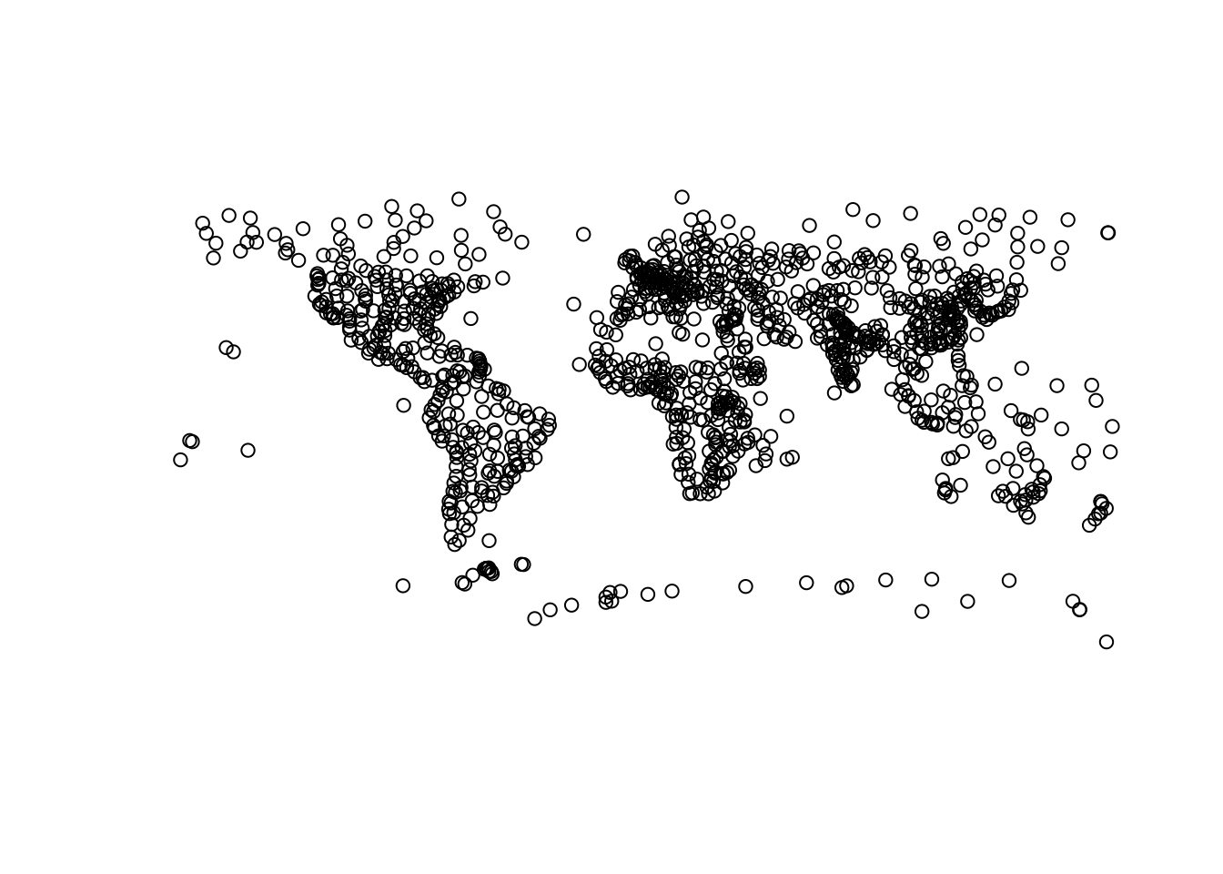
url_popplaces = (
    "https://raw.githubusercontent.com/nvkelso/natural-earth-vector/"
    "master/geojson/ne_50m_populated_places_simple.geojson"
)

# Read GeoJSON data directly from the URL
populated_places = gpd.read_file(url_popplaces)

# Plotting the data
fig, ax = plt.subplots(figsize=(12, 8))
populated_places.plot(ax=ax, marker='o', color='black', markersize=10, alpha=0.5)
ax.set_title('Populated Places of the World')
plt.show()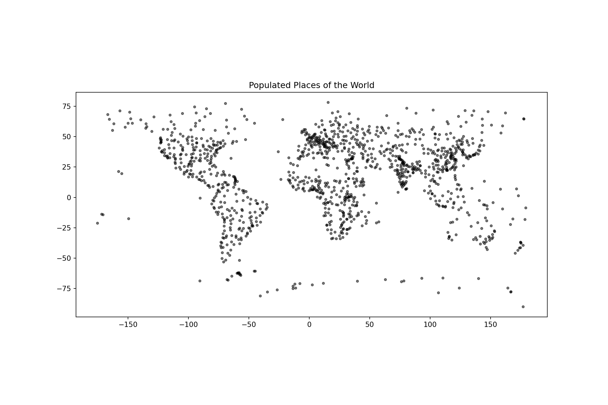
Note the code cell above requires internet connectivity.
Now we subset to India only — this leaves us with 71 places to work with:
places <- data %>%
  filter(adm0name == "India")
places = populated_places.query("adm0name == 'India'")By default, place locations come expressed in longitude and latitude. Because you will be working with distances, it makes sense to convert the table into a system expressed in metres. For India, this can be the “Kalianpur 1975 / India zone I” (EPSG:24378) projection.
places_m <- st_transform(places, crs = 24378)places_m = places.to_crs(epsg=24378)This is what we have to work with then:
ggplot() +
  geom_sf(data = places_m, aes(size = pop_max), colour = "goldenrod", alpha = 0.7) +
  scale_size_continuous(name = "Population", range = c(1, 9), labels = scales::comma) +
  ggtitle("Populated places in India") +
  theme_void()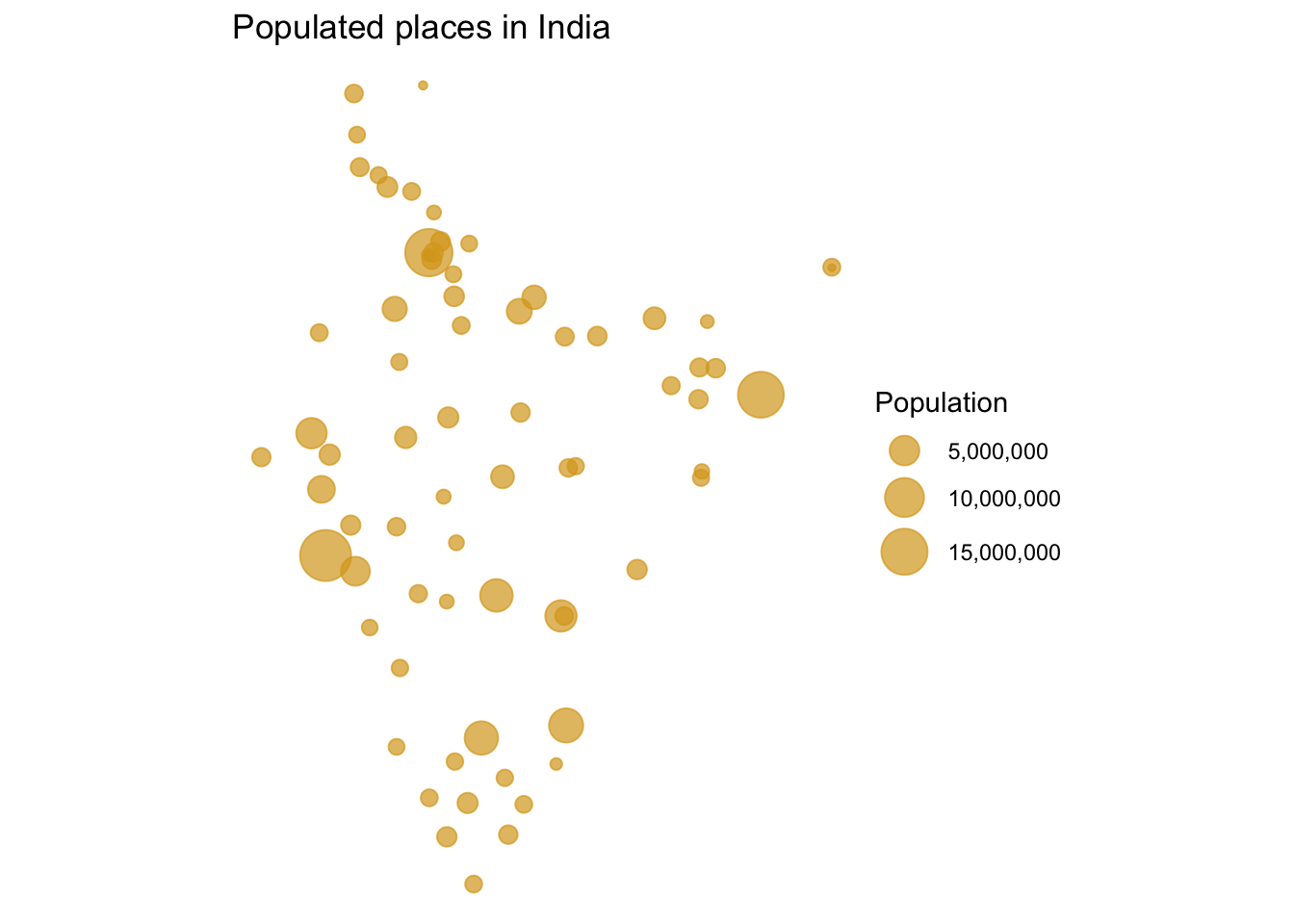
ax = places_m.plot(
    color="xkcd:bright yellow", markersize=places_m["pop_max"] / 50000,
    alpha=0.7, figsize=(9, 9)
)
cx.add_basemap(
    ax,
    crs=places_m.crs,
    source=cx.providers.Esri.WorldGrayCanvas
)
ax.set_title("Populated places in India")
ax.set_axis_off()
plt.show()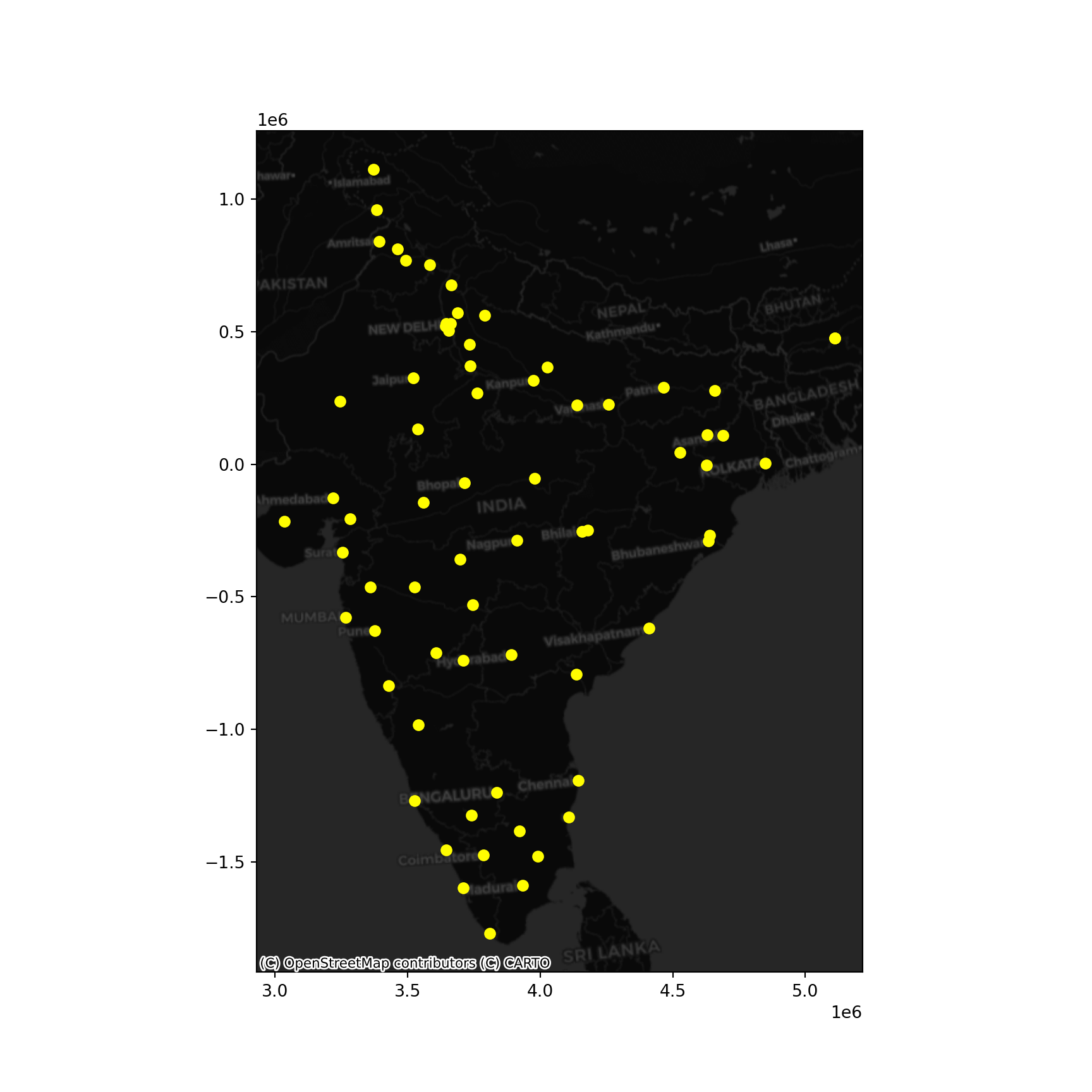
With this at hand, get to work:
Use the DBSCAN algorithm to identify clusters
Start with the following parameters: at least five cities for a cluster (min_samples) and a maximum of 1,000Km (eps)
Obtain the clusters and plot them on a map. Does it pick up any interesting pattern?
Based on the results above, tweak the values of both parameters to find a cluster of southern cities, and another one of cities in the North around New Dehli