2  Lab: Exploring a Dataset

Author

Gabriele Filomena

Published

October 5, 2026

The following material has been readapted from:

The lecture’s slides can be found here.

Before completing the practical, please take this quiz.

Open this lab in RStudio: in the Files pane, click labs and then 01.DataExploration.qmd. Save your own copy in myLabs (File -> Save As...) and work on the copy. Work through it from top to bottom, running each code chunk and adding your notes and answers in the file. (First time? See the Setup guide, then do Lab: Introduction to R, which shows how to run code chunks.)

Follow the practical below. You can describe what you are doing in normal text. See here for how to format normal text in Markdown documents.

2.1 Practice: Dataset and Dataframes

Within this module we will be working with data stored in so-called datasets. A dataset is a structured collection of data points that represent various measurements or observations, often organized in a tabular format with rows and columns. A dataset might contain information about different locations, such as neighborhoods or cities, with each row representing a place and each column detailing characteristics like population density, average income, or number of green parks. For example, a dataset could be compiled to study patterns in urban mobility, where the data includes the number of daily commuters, the distance they travel, and the mode of transport they use. Datasets provide the essential building blocks for statistical analysis; they enable exploring relationships, identifying patterns, and drawing conclusions about certain phenomena.

Examples of everyday datasets:

  • Premier League Standings: Each row represents a team, with columns for points, games played, wins, draws, and losses.
  • Movie Dataset: Each row represents a movie, with columns showing its title, genre, release year, director, and rating.
  • Weather Dataset: Each row shows a day’s weather in a city, with columns for temperature, humidity, wind speed, and precipitation.

Usually, data is organized in

  • Columns of data representing some trait or variable that we might be interested in. In general, we might wish to investigate the relationship between variables.
  • Rows represent a single object on which the column traits are measured.

For example, in a grade book for recording students scores throughout the semester, there is one row for every student and columns for each assignment. A greenhouse experiment dataset will have a row for every plant and columns for treatment type and biomass.

2.1.1 Datasets in R

In R, we want a way of storing data where it feels just as if we had an Excel Spreadsheet where each row represents an observation and each column represents some information about that observation. We will call this object a data.frame, an R representation of a data set. The easiest way to understand data frames is to create one.

Task: Run the chunk below. It creates a data.frame that represents an instructor’s grade book, where each row is a student, and each column represents some sort of assessment.

library(dplyr)

Grades <- data.frame(
  Name  = c('Bob','Jeff','Mary','Valerie'),     
  Exam.1 = c(90, 75, 92, 85),
  Exam.2 = c(87, 71, 95, 81)
)
# Show the data.frame 
# View(Grades)  # show the data in an Excel-like tab.  Doesn't work when knitting 
Grades          # show the output in the console. This works when knitting
     Name Exam.1 Exam.2
1     Bob     90     87
2    Jeff     75     71
3    Mary     92     95
4 Valerie     85     81

R allows two different ways to access elements of the data.frame. First is a matrix-like notation for accessing particular values.

Format Result
[a,b] Element in row a and column b
[a,] All of row a
[,b] All of column b

Because the columns have meaning and we have given them column names, it is desirable to want to access an element by the name of the column as opposed to the column number.

Task: Run:

Grades[, 2]       # print out all of column 2 
[1] 90 75 92 85
Grades$Name       # The $-sign means to reference a column by its label
[1] "Bob"     "Jeff"    "Mary"    "Valerie"

2.1.2 Importing Data in R

Usually we won’t type the data in by hand, but rather load the data from some package. Reading data from external sources is a necessary skill.

Comma Separated Values Data

To consider how data might be stored, we first consider the simplest file format: the comma separated values file (.csv). In this file type, each of the “cells” of data are separated by a comma. For example, the data file storing scores for three students might be as follows:

Able, Dave, 98, 92, 94
Bowles, Jason, 85, 89, 91
Carr, Jasmine, 81, 96, 97

Typically when you open up such a file on a computer with MS Excel installed, Excel will open up the file assuming it is a spreadsheet and put each element in its own cell. However, you can also open the file using a more primitive program (say Notepad in Windows, TextEdit on a Mac) you’ll see the raw form of the data.

Having just the raw data without any sort of column header is problematic (which of the three exams was the final??). Ideally we would have column headers that store the name of the column.

LastName, FirstName, Exam1, Exam2, FinalExam
Able, Dave, 98, 92, 94
Bowles, Jason, 85, 89, 91
Carr, Jasmine, 81, 96, 97

Reading (.csv) files

To make R read in the data arranged in this format, we need to tell R three things:

  1. Where does the data live? Often this will be the name of a file on your computer, but the file could just as easily live on the internet (provided your computer has internet access).

  2. Is the first row data or is it the column names?

  3. What character separates the data? Some programs store data using tabs to distinguish between elements, some others use white space. R’s mechanism for reading in data is flexible enough to allow you to specify what the separator is.

The primary function that we’ll use to read data from a file and into R is the function read.csv(). This function has many optional arguments but the most commonly used ones are outlined in the table below.

Argument Default Description
file Required A character string denoting the file location.
header TRUE Specifies whether the first line contains column headers.
sep "," Specifies the character that separates columns. For read.csv(), this is usually a comma.
skip 0 The number of lines to skip before reading data; useful for files with descriptive text before the actual data.
na.strings "NA" Values that represent missing data; multiple values can be specified, e.g., c("NA", "-9999").
quote " Specifies the character used to quote character strings, typically " or '.
stringsAsFactors FALSE Controls whether character strings are converted to factors; FALSE means they remain as character data.
row.names NULL Allows specifying a column as row names, or assigning NULL to use default indexing for rows.
colClasses NULL Specifies the data type for each column to speed up reading for large files, e.g., c("character", "numeric").
encoding "unknown" Sets the text encoding of the file, which can be useful for files with special or international characters.

Most of the time you just need to specify the file.

Task: Let’s read in a dataset of terrorist attacks that have taken place in the UK:

attacks <- read.csv(file   = '../data/attacksUK.csv')  # where the data lives                                 
View(attacks)

2.2 Practice: Descriptive Statistics

2.2.1 Summarizing Data

It is very important to be able to take a data set and produce summary statistics such as the mean and standard deviation of a column. For this sort of manipulation, we use the package dplyr. This package allows chaining together many common actions to form a particular task.

The fundamental operations to perform on a data set are:

  • Subsetting - Returns a dataframe with only particular columns or rows

    – select - Selecting a subset of columns by name or column number.

    – filter - Selecting a subset of rows from a data frame based on logical expressions.

    – slice - Selecting a subset of rows by row number.

  • arrange - Re-ordering the rows of a data frame.

  • mutate - Add a new column that is some function of other columns.

  • summarise - calculate some summary statistic of a column of data. This collapses a set of rows into a single row.

Each of these operations is a function in the package dplyr. These functions all have a similar calling syntax:

  • The first argument is a data set.

  • Subsequent arguments describe what to do with the input data frame and you can refer to the columns without using the df$column notation.

All of these functions will return a data set.

Let’s consider the summarise function to calculate the mean score for Exam.1. Notice that this takes a data frame of four rows, and summarizes it down to just one row that represents the summarized data for all four students.

library(dplyr) # load the library
Grades %>%
  summarize( Exam.1.mean = mean( Exam.1 ) )
  Exam.1.mean
1        85.5

Similarly you could calculate the standard deviation for the exam as well.

Grades %>%
  summarize( Exam.1.mean = mean( Exam.1 ),
             Exam.1.sd   = sd(   Exam.1   ) )
  Exam.1.mean Exam.1.sd
1        85.5  7.593857

Task: Insert a new chunk below and calculate the mean and standard deviation of Exam.2. Type the code yourself instead of copying it: it is the best way to learn it.

The %>% operator works by translating the command a %>% f(b) to the expression f(a,b). This operator works on any function f. This is useful when we want to start with x, and first apply a function f(), then g(), and then h(); the usual R command would be h(g(f(x))) which is hard to read. Using the pipe command %>%, this sequence of operations becomes x %>% f() %>% g() %>% h().

Below, the code takes the Grades dataframe and calculates a column for the average exam score, and then sorts the data according to that average score

Grades %>%   mutate( Avg.Score = (Exam.1 + Exam.2) / 2 ) %>%   arrange( Avg.Score )
     Name Exam.1 Exam.2 Avg.Score
1    Jeff     75     71      73.0
2 Valerie     85     81      83.0
3     Bob     90     87      88.5
4    Mary     92     95      93.5

You don’t have to memorise this.

Let’s go back to the terrorist attacks dataframe. There are attacks perpetrated by several different groups. Each record is a single attack and contains information about who perpetrated the attack, what year, how many were killed and how many were wounded. You can get a glimpse of the dataframe with the function head

head(attacks, n = 10)
   nrKilled nrWound year        country                        group
1         0       0 2005 United Kingdom   Abu Hafs al-Masri Brigades
2         0       0 2005 United Kingdom   Abu Hafs al-Masri Brigades
3         0       0 2005 United Kingdom   Abu Hafs al-Masri Brigades
4         0       0 2005 United Kingdom   Abu Hafs al-Masri Brigades
5         0       1 1982 United Kingdom Abu Nidal Organization (ANO)
6         0       0 2014 United Kingdom                   Anarchists
7         0       0 2014 United Kingdom                   Anarchists
8         0       0 2014 United Kingdom                   Anarchists
9         0       0 2014 United Kingdom                   Anarchists
10        0       0 2014 United Kingdom                   Anarchists
                           attack                      target
1               Bombing/Explosion              Transportation
2               Bombing/Explosion              Transportation
3               Bombing/Explosion              Transportation
4               Bombing/Explosion              Transportation
5                   Assassination     Government (Diplomatic)
6  Facility/Infrastructure Attack                    Business
7  Facility/Infrastructure Attack                    Business
8  Facility/Infrastructure Attack                    Business
9  Facility/Infrastructure Attack Private Citizens & Property
10 Facility/Infrastructure Attack                      Police
                      weapon
1  Explosives/Bombs/Dynamite
2  Explosives/Bombs/Dynamite
3  Explosives/Bombs/Dynamite
4  Explosives/Bombs/Dynamite
5                   Firearms
6                 Incendiary
7                 Incendiary
8                 Incendiary
9                 Incendiary
10                Incendiary

We might want to compare different actors and see the mean and standard deviation of the number of people wounded, by each group’s attack, across time. To do this, we are still going to use summarise(), but we will precede it with group_by(group) to tell the subsequent dplyr functions to perform the actions separately for each group.

attacks %>%
  group_by( group) %>%
  summarise( Mean = mean(nrWound), 
             Std.Dev = sd(nrWound))
# A tibble: 38 × 3
   group                                                Mean Std.Dev
   <chr>                                               <dbl>   <dbl>
 1 Abu Hafs al-Masri Brigades                         0        0    
 2 Abu Nidal Organization (ANO)                       1       NA    
 3 Anarchists                                         0        0    
 4 Animal Liberation Front (ALF)                      0.0833   0.282
 5 Animal Rights Activists                            0.167    0.389
 6 Armenian Secret Army for the Liberation of Armenia 0.2      0.447
 7 Black September                                    0.667    0.577
 8 Continuity Irish Republican Army (CIRA)            0.7      3.12 
 9 Dissident Republicans                              0.0758   0.267
10 Informal Anarchist Federation                      0        0    
# ℹ 28 more rows

Task: Run the chunk above. Then insert a new chunk and try out another categorical variable instead of group (e.g. year) and nrKilled instead of nrWound.

Let’s now move to another dataset to address a research question.

For illustration purposes, we will use the Family Resources Survey (FRS). The FRS is an annual survey conducted by the UK government that collects detailed information about the income, living conditions, and resources of private households across the United Kingdom. Managed by the Department for Work and Pensions (DWP), the FRS provides data that is essential for understanding the economic and social conditions of households and informing public policy.

Consider questions such as:

  • How many respondents (persons) are there in the 2016-17 FRS?
  • How many variables (population attributes) are there?
  • What types of variables are present in the FRS?
  • What is the most detailed geography available in the FRS?

Task: To answer these questions, download FRS16-17_labels.csv from the FRS page on Canvas and upload it to a new folder data/FRS in RStudio (see Setup, section 5). Then load and inspect the dataset.

# the FRS dataset should be already loaded, otherwise
frs_data <- read.csv("../data/FRS/FRS16-17_labels.csv") 

# Display basic structure 
glimpse(frs_data)
Rows: 44,145
Columns: 45
$ household        <int> 6087, 6101, 6103, 6122, 6134, 6136, 6138, 6140, 6143,…
$ family           <int> 1, 1, 1, 1, 1, 1, 1, 1, 1, 1, 1, 1, 1, 1, 1, 1, 1, 1,…
$ person           <int> 5, 3, 3, 3, 2, 4, 4, 3, 3, 4, 4, 3, 4, 2, 5, 3, 4, 3,…
$ country          <chr> "England", "England", "England", "Northern Ireland", …
$ region           <chr> "London", "South East", "Yorks and the Humber", "Nort…
$ age_group        <chr> "05-10", "05-10", "05-10", "05-10", "05-10", "05-10",…
$ sex              <chr> "Female", "Male", "Male", "Female", "Female", "Female…
$ marital_status   <chr> "Single", "Single", "Single", "Single", "Single", "Si…
$ ethnicity        <chr> "Mixed / multiple ethnic groups", "White", "White", "…
$ hrp              <chr> "Not HRP", "Not HRP", "Not HRP", "Not HRP", "Not HRP"…
$ rel_to_hrp       <chr> "Son/daughter (incl. adopted)", "Son/daughter (incl. …
$ lifestage        <chr> "Child (0-17)", "Child (0-17)", "Child (0-17)", "Chil…
$ dependent        <chr> "Dependent", "Dependent", "Dependent", "Dependent", "…
$ arrival_year     <chr> "UK Born", "UK Born", "UK Born", "UK Born", "UK Born"…
$ birth_country    <chr> "Dependent child", "Dependent child", "Dependent chil…
$ care_hours       <chr> "0 hours per week", "0 hours per week", "0 hours per …
$ educ_age         <chr> "Dependent child", "Dependent child", "Dependent chil…
$ educ_type        <chr> "School (full-time)", "School (full-time)", "School (…
$ fam_youngest     <chr> "7", "4", "0", "7", "0", "9", "10", "0", "3", "10", "…
$ fam_toddlers     <int> 0, 1, 1, 0, 2, 0, 0, 2, 1, 0, 0, 1, 0, 1, 0, 0, 0, 1,…
$ fam_size         <int> 4, 4, 4, 3, 4, 4, 3, 5, 4, 4, 3, 4, 4, 3, 5, 4, 4, 4,…
$ happy            <chr> "Dependent child", "Dependent child", "Dependent chil…
$ health           <chr> "Not known", "Not known", "Not known", "Not known", "…
$ hh_accom_type    <chr> "Terraced house/bungalow", "Detached house/bungalow",…
$ hh_benefits      <int> 10868, 0, 1768, 8632, 8372, 1768, 1768, 1768, 0, 0, 1…
$ hh_composition   <chr> "Three or more adults, 1+ children", "One adult femal…
$ hh_ctax_band     <chr> "Band D", "Band F", "Band A", "Band B", "Band A", "Ba…
$ hh_housing_costs <chr> "4316", "10296", "5408", "Northern Ireland", "5720", …
$ hh_income_gross  <int> 54236, 180804, 26936, 19968, 17992, 76596, 31564, 366…
$ hh_income_net    <int> 44668, 120640, 23556, 19968, 17992, 62868, 29744, 287…
$ hh_size          <int> 5, 4, 4, 3, 4, 4, 4, 5, 4, 4, 4, 4, 4, 5, 5, 4, 4, 4,…
$ hh_tenure        <chr> "Mortgaged (including part rent / part own)", "Mortga…
$ highest_qual     <chr> "Dependent child", "Dependent child", "Dependent chil…
$ income_gross     <int> 0, 0, 0, 0, 0, 0, 0, 0, 0, 0, 0, 0, 0, 0, 0, 0, 0, 0,…
$ income_net       <int> 0, 0, 0, 0, 0, 0, 0, 0, 0, 0, 0, 0, 0, 0, 0, 0, 0, 0,…
$ jobs             <chr> "Dependent child", "Dependent child", "Dependent chil…
$ life_satisf      <chr> "Dependent child", "Dependent child", "Dependent chil…
$ nssec            <chr> "Dependent child", "Dependent child", "Dependent chil…
$ sic_chapter      <chr> "Dependent child", "Dependent child", "Dependent chil…
$ sic_division     <chr> "Dependent child", "Dependent child", "Dependent chil…
$ soc2010          <chr> "Dependent child", "Dependent child", "Dependent chil…
$ work_hours       <chr> "Dependent child", "Dependent child", "Dependent chil…
$ workstatus       <chr> "Dependent Child", "Dependent Child", "Dependent Chil…
$ years_ft_work    <chr> "Dependent child", "Dependent child", "Dependent chil…
$ survey_weight    <int> 2315, 1317, 2449, 427, 1017, 1753, 1363, 1344, 828, 1…
and summary:

summary(frs_data)
   household         family          person       country         
 Min.   :    1   Min.   :1.000   Min.   :1.00   Length:44145      
 1st Qu.: 4816   1st Qu.:1.000   1st Qu.:1.00   Class :character  
 Median : 9673   Median :1.000   Median :2.00   Mode  :character  
 Mean   : 9677   Mean   :1.106   Mean   :1.98                     
 3rd Qu.:14553   3rd Qu.:1.000   3rd Qu.:3.00                     
 Max.   :19380   Max.   :6.000   Max.   :9.00                     
    region           age_group             sex            marital_status    
 Length:44145       Length:44145       Length:44145       Length:44145      
 Class :character   Class :character   Class :character   Class :character  
 Mode  :character   Mode  :character   Mode  :character   Mode  :character  


  ethnicity             hrp             rel_to_hrp         lifestage        
 Length:44145       Length:44145       Length:44145       Length:44145      
 Class :character   Class :character   Class :character   Class :character  
 Mode  :character   Mode  :character   Mode  :character   Mode  :character  


  dependent         arrival_year       birth_country       care_hours       
 Length:44145       Length:44145       Length:44145       Length:44145      
 Class :character   Class :character   Class :character   Class :character  
 Mode  :character   Mode  :character   Mode  :character   Mode  :character  


   educ_age          educ_type         fam_youngest        fam_toddlers   
 Length:44145       Length:44145       Length:44145       Min.   :0.0000  
 Class :character   Class :character   Class :character   1st Qu.:0.0000  
 Mode  :character   Mode  :character   Mode  :character   Median :0.0000  
                                                          Mean   :0.2557  
                                                          3rd Qu.:0.0000  
                                                          Max.   :4.0000  
    fam_size        happy              health          hh_accom_type     
 Min.   :1.000   Length:44145       Length:44145       Length:44145      
 1st Qu.:2.000   Class :character   Class :character   Class :character  
 Median :2.000   Mode  :character   Mode  :character   Mode  :character  
 Mean   :2.599                                                           
 3rd Qu.:4.000                                                           
 Max.   :9.000                                                           
  hh_benefits    hh_composition     hh_ctax_band       hh_housing_costs  
 Min.   :    0   Length:44145       Length:44145       Length:44145      
 1st Qu.:    0   Class :character   Class :character   Class :character  
 Median : 1768   Mode  :character   Mode  :character   Mode  :character  
 Mean   : 5670                                                           
 3rd Qu.:10192                                                           
 Max.   :54080                                                           
 hh_income_gross   hh_income_net        hh_size      hh_tenure        
 Min.   :-326092   Min.   :-334776   Min.   :1.00   Length:44145      
 1st Qu.:  22256   1st Qu.:  20748   1st Qu.:2.00   Class :character  
 Median :  35984   Median :  31512   Median :3.00   Mode  :character  
 Mean   :  46076   Mean   :  37447   Mean   :2.96                     
 3rd Qu.:  57252   3rd Qu.:  47008   3rd Qu.:4.00                     
 Max.   :1165216   Max.   :1116596   Max.   :9.00                     
 highest_qual        income_gross       income_net          jobs          
 Length:44145       Min.   :-354848   Min.   :-358592   Length:44145      
 Class :character   1st Qu.:     52   1st Qu.:      0   Class :character  
 Mode  :character   Median :  12740   Median :  12012   Mode  :character  
                    Mean   :  17305   Mean   :  14204                     
                    3rd Qu.:  23712   3rd Qu.:  20384                     
                    Max.   :1127360   Max.   :1110928                     
 life_satisf           nssec           sic_chapter        sic_division      
 Length:44145       Length:44145       Length:44145       Length:44145      
 Class :character   Class :character   Class :character   Class :character  
 Mode  :character   Mode  :character   Mode  :character   Mode  :character  


   soc2010           work_hours         workstatus        years_ft_work     
 Length:44145       Length:44145       Length:44145       Length:44145      
 Class :character   Class :character   Class :character   Class :character  
 Mode  :character   Mode  :character   Mode  :character   Mode  :character  


 survey_weight  
 Min.   :  221  
 1st Qu.: 1097  
 Median : 1380  
 Mean   : 1459  
 3rd Qu.: 1742  
 Max.   :39675  

2.2.2 Understanding the Structure of the FRS Datafile

In the FRS data structure, each row represents a person, but:

  • Each person is nested within a family.
  • Each family is nested within a household.

Below is an example dataset structure:

household family person region age_group sex marital_status rel_to_hrp
1 1 1 London 40-44 Female Married/Civil partnership Spouse
1 1 2 London 40-44 Male Married/Civil partnership Household Representative
1 1 3 London 5-10 Male Single Son/daughter (incl. adopted)
1 1 4 London 5-10 Female Single Son/daughter (incl. adopted)
1 1 5 London 16-19 Male Single Step-son/daughter
2 1 1 Scotland 35-39 Male Single Household Representative
3 1 1 Yorks and the Humber 35-39 Female Married/Civil partnership Household Representative
3 1 2 Yorks and the Humber 35-39 Male Married/Civil partnership Spouse
3 1 3 Yorks and the Humber 5-10 Male Single Step-son/daughter
4 1 1 Wales 0-4 Male Single Son/daughter (incl. adopted)
4 1 2 Wales 60-64 Male Married/Civil partnership Household Representative
4 1 3 Wales 55-59 Female Married/Civil partnership Spouse
4 2 3 Wales 30-34 Female Single Son/daughter (incl. adopted)

The first five people in the FRS all belong to the same household (household 1); they also all belong to the same family. This family comprises a married middle-aged couple plus their three children, one of whom is a stepson.

The second household (household 2) comprises only one person – a single middle-aged male.The third household comprises another married couple, this time with two children.

Superficially the fourth household looks similar to households 1 and 2: a married couple plus their daughter. The difference is that this particular married couple is nearing retirement age, and their daughter is middle-aged. Consequently, despite being a child of the married couple, the middle-aged daughter is treated as a separate ‘family’ (family 2 in the household). This is because the FRS (and Census) define a ‘family’ as a couple plus any ‘dependent’ children. A dependent child is defined as a child who is either aged 0-15 or aged 16-19, unmarried and in full-time education. All children aged 16-19 who are married or no longer in full-time education are regarded as ‘independent’ adults who form their own family unit, as are all children aged 20+.

The inclusion of all persons in a household allows us more flexibility in the types of research question we can answer. For example, we could explore how the likelihood of a woman being in paid employment WorkStatus is influenced by the age of the youngest child still living in her family (if any) fam_youngest.

In the FRS (and Census), a “family” is defined as a couple and any “dependent” children. Dependent children are defined as those aged 0–15, or aged 16–19 if unmarried and in full-time education.

2.2.3 Explore the Distribution of Your Outcome Variable

Before starting your analysis, it is critical to know the type of scale used to measure your outcome variable: is it categorical or continuous? Here we will start off by exploring a continuous variable which can then turn into a categorical variable (e.g. top earners: yes or no). We explore the income distribution in the UK by first looking at the low and high end of the distribution ie. What sorts of people have high (or low) incomes?

In the FRS each person’s annual income is recorded, both gross (pre-tax) and net (post-tax). This income includes all income sources, including earnings, profits, investment returns, state benefits, occupational pensions etc. As it is possible to make a loss on some of these activities, it is also possible (although unusual) for someone’s gross or net annual income in a given year to be negative (representing an overall loss).

Task: Load the FRS dataset into your R environment, if it’s not already loaded, and inspect the data.

Open the dataset in RStudio’s Data Viewer to explore its structure, including the income_gross and income_net variables.

 # Open the data in the RStudio Viewer
View(frs_data)

in the Data Viewer tab, scroll horizontally to locate the income_gross and income_net columns. If columns are listed alphabetically, they will appear near other attributes that start with “income.”

You should notice two things:

  • Incomes are recorded to the nearest £, NOT in income bands.
  • Dependent children almost all have a recorded income of £0.

This second observation highlights the somewhat loose wording of our question above (What sorts of people have high (or low) incomes?). To avoid reaching the somewhat banal conclusion that those with the lowest of all incomes are almost all children, we should re-frame the question more precisely as What sorts of people (excluding dependent children) have low incomes?

Task: Determine the Scale of the Outcome Variable.

# Summarize income variables
summary(frs_data$income_gross)
   Min. 1st Qu.  Median    Mean 3rd Qu.    Max. 
-354848      52   12740   17305   23712 1127360 
# Summarize income variables
summary(frs_data$income_net)
   Min. 1st Qu.  Median    Mean 3rd Qu.    Max. 
-358592       0   12012   14204   20384 1110928 

Task: Exclude Dependent Children.

You need to select all cases (persons) that are independent, that is where the variable dependent has values different from != “Dependent” or equal == “Independent”.

# Filter to include only independent persons
frs_independent <- frs_data %>% filter(dependent != "Dependent")

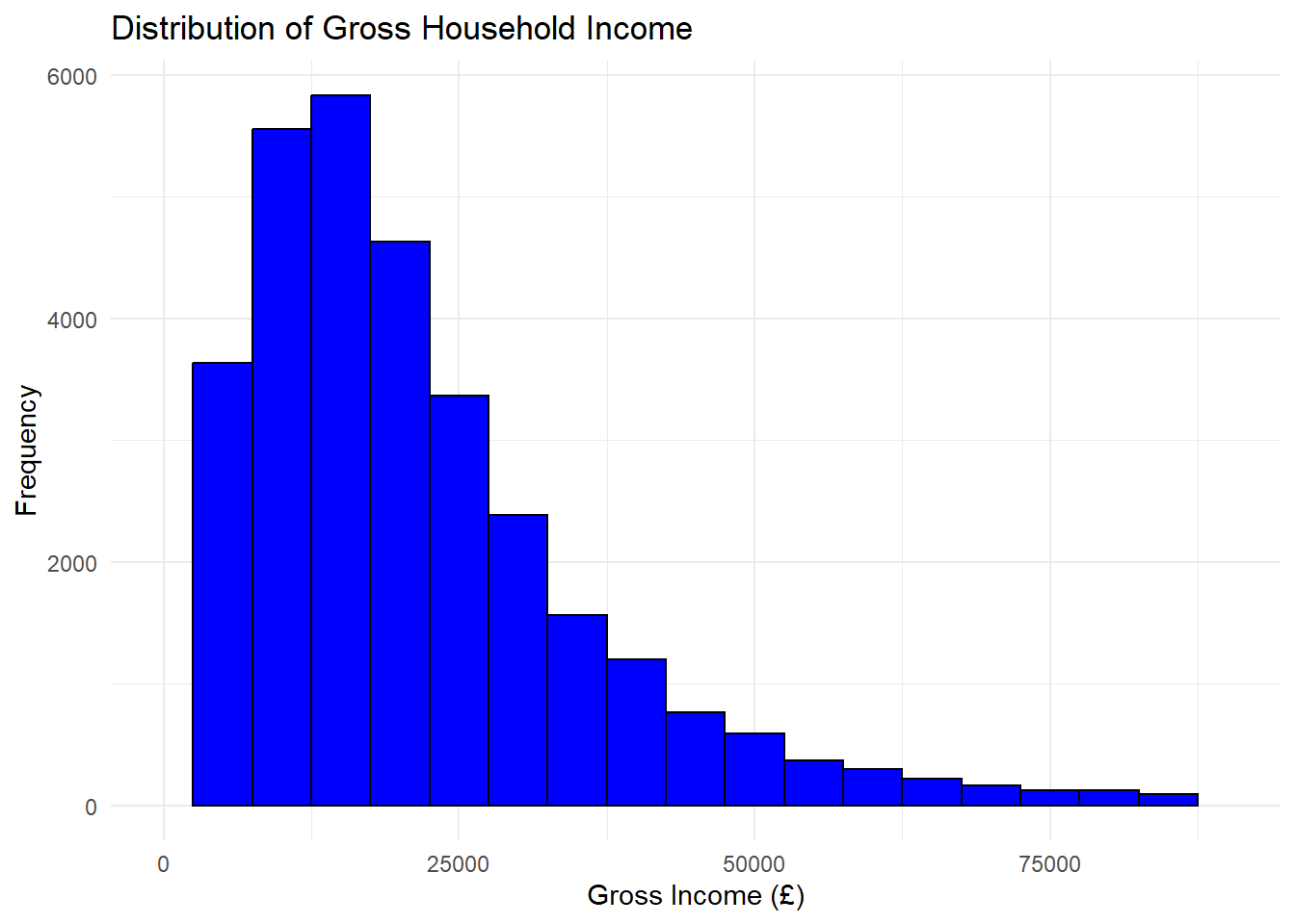
Task: Create a basic histogram (a visualisation lecture is scheduled later on).

The income variables in the FRS are all scale variables so a good starting point is to examine its distribution looking at a histogram of income_gross.

library(ggplot2)
 
 ggplot(frs_independent, aes(x = income_gross)) +
   geom_histogram(binwidth = 5000, fill = "blue", color = "black") +
   labs(
     title = "Distribution of Gross Household Income",
     x = "Gross Income (£)",
     y = "Frequency"
   ) +
   xlim(0, 90000) +
   theme_minimal()

You should see the histogram below. It reveals that the income distribution is very skewed with few people earning high salaries and the majority earning just over or less 35,000 annually.

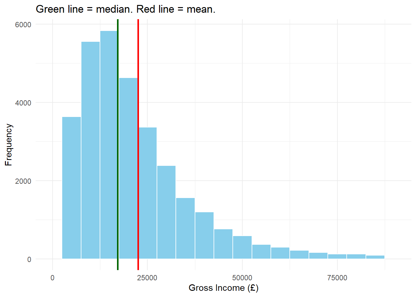
Why this matters: the mean and the median disagree.

Look back at the summary() output. The mean gross income is about £22,544, but the median is about £17,108 — a difference of more than £5,000. Both are “the average”. Both are correct. So which one should you report?

The histogram answers it. Let’s draw the two numbers onto it:

ggplot(frs_independent, aes(x = income_gross)) +
  geom_histogram(binwidth = 5000, fill = "skyblue", color = "white") +
  geom_vline(xintercept = median(frs_independent$income_gross), colour = "darkgreen", linewidth = 1) +
  geom_vline(xintercept = mean(frs_independent$income_gross), colour = "red", linewidth = 1) +
  labs(
    title = "Green line = median. Red line = mean.",
    x = "Gross Income (£)",
    y = "Frequency"
  ) +
  xlim(0, 90000) +
  theme_minimal()

geom_vline() simply draws a vertical line at the position you give it. Here we give it the median and the mean.

The green median line sits in the middle of the tall bars, where most people actually are. The red mean line sits noticeably to the right, in a region where comparatively few people are. Nobody moved it there deliberately: the mean is dragged upwards by the long tail of very high earners off to the right of the chart (remember, the highest income in this dataset is over £1,000,000). The median cannot be dragged like this, because it only cares about who is in the middle of the queue, not how rich the richest person is.

Task: Which of the two lines better describes “a typical person’s income” in this dataset? This is not a trick question — look at where the bars are.

This is why income, house prices and similar skewed variables are almost always reported as medians, and it is a point worth making in your assignment if you use one of them. It is also a warning: whenever you report a mean, look at the histogram first. If the distribution has a long tail, the mean is describing the tail as much as it is describing your typical case.

Task: Adopt a regrouping strategy.

You can also cross-tabulate gross (or net) income with any of the other variables in the FRS to your heart’s content – or can you?

Again, here is important to recall that the income variables in the FRS are all ‘scale’ variables; in other words, they are precise measures rather than broad categories. Consequently, every single person in the FRS potentially has their own unique income value. That could make for a table c. 44,000 rows long (one row per person) if each person has their own unique value. The solution is to create a categorical version of the original income variable by assigning each person to one of a set of income categories (income bands). Having done this, cross-tabulation then becomes possible.

But which strategy to use? Equal intervals, percentiles or ‘ad hoc’. Here I would suggest that ‘ad hoc’ is best: all you want to do is to allocate each independent adult to one of three arbitrarily defined groups: ‘low’, ‘middle’ and ‘high’ income. Define Low and High Income Thresholds

Define thresholds for income categories:

  • Low-income threshold: £________
  • High-income threshold: £_______

Task: Create a New Variable Based on Regrouping of Original Variable.

Recode income_gross into categories based on the chosen thresholds.

# Define thresholds for income categories 
LOW_THRESHOLD <- 10000 # Replace with the upper limit for low income 
HIGH_THRESHOLD <- 50000 # Replace with the lower limit for high income 

# Define income categories based on thresholds 
frs_independent <- frs_independent %>% 
    mutate(income_category = case_when( 
        income_gross <= LOW_THRESHOLD ~ "Low", 
        income_gross >= HIGH_THRESHOLD ~ "High", 
        TRUE ~ "Middle" ))

Before looking at the results, it is worth seeing what you have just done to the data. The two thresholds are simply two lines drawn across the distribution:

ggplot(frs_independent, aes(x = income_gross)) +
  geom_histogram(binwidth = 5000, fill = "grey80", color = "white") +
  geom_vline(xintercept = LOW_THRESHOLD, colour = "red", linewidth = 1) +
  geom_vline(xintercept = HIGH_THRESHOLD, colour = "red", linewidth = 1) +
  labs(
    title = "Your two thresholds, drawn on the distribution",
    subtitle = "Everything left of the first line is 'Low'. Everything right of the second is 'High'.",
    x = "Gross Income (£)",
    y = "Frequency"
  ) +
  xlim(0, 90000) +
  theme_minimal()

Notice how much of the population falls between the lines, and how little falls beyond the right-hand one. Now change LOW_THRESHOLD to 15000, re-run both chunks, and watch the red line move and the “Low” group grow.

Task: There is no correct answer here, and that is the point. You chose those two numbers, and your choice decides who counts as poor and who counts as rich. If you recode a variable like this in your assignment, you must say what thresholds you used and why — the marking criteria ask for exactly that.

The mutate() function in R, from the dplyr package, is used to add or modify columns in a data frame. It allows you to create new variables or transform existing ones by applying calculations or conditional statements directly within the function.

Explanation of the code

  • frs_independent %>%: The pipe operator %>% sends frs_independent into mutate(), allowing us to apply transformations without reassigning it repeatedly.
  • mutate(): Starts the transformation process by defining new or modified columns.
  • income_category = case_when(...):
    • This creates a new column named income_category.
    • The case_when() function defines conditions for assigning values to this new column.
  • case_when():
    • case_when() is used here to assign categorical labels based on conditions.
    • income_gross <= LOW_THRESHOLD ~ "Low": If income_gross is less than or equal to LOW_THRESHOLD, income_category will be labeled “Low.”
    • income_gross >= HIGH_THRESHOLD ~ "High": If income_gross is greater than or equal to HIGH_THRESHOLD, income_category will be labeled “High.”
    • TRUE ~ "Middle": Any values not meeting the previous conditions are labeled “Middle.”

Task: Add some Metadata.

Define metadata for the new variable by labeling income categories.

# Add metadata by converting to a factor and defining labels

frs_independent$income_category <- factor(frs_independent$income_category,
                        levels = c("Low", "Middle", "High"), labels = c("<= £10,000", "£10,001 - £49,999", ">= £50,000"))

Task: Check your work.

Examine the frequency distribution of the variable you have just created. Both variables should have the same number of missing cases, unless:

  • Missing cases in the old variable have been intentionally converted into valid cases in the new variable.
  • You forgot to allocate a new value to one of the old variable categories, in which case the new variable will have more missing cases than the old variable.
# Frequency distribution of income categories
table(frs_independent$income_category)

       <= £10,000 £10,001 - £49,999        >= £50,000 
             8584             22981              2271 

After preparing the data, use cross-tabulations to compare income levels across demographic groups.

# Cross-tabulate income category by age group, nationality, etc.
table(frs_independent$income_category, frs_independent$age_group)
                   
                    16-19 20-24 25-29 30-34 35-39 40-44 45-49 50-54 55-59 60-64
  <= £10,000          373   680   492   558   474   511   554   652   781   826
  £10,001 - £49,999   263  1241  1802  2056  2052  1948  1995  1967  1749  1772
  >= £50,000            1     8    59   186   314   331   334   356   237   177
                   
                    65-69 70-74  75+
  <= £10,000          773   744 1166
  £10,001 - £49,999  2073  1554 2509
  >= £50,000          144    56   68

Explore income distribution across different regions.

# Cross-tabulate income category by region
table(frs_independent$income_category, frs_independent$region) 
                   
                    East Midlands East of England London North East North West
  <= £10,000                  562             665    740        357        878
  £10,001 - £49,999          1550            1855   1850        979       2347
  >= £50,000                  135             245    367         48        174
                   
                    Northern Ireland Scotland South East South West Wales
  <= £10,000                     874     1212        895        588   399
  £10,001 - £49,999             2305     3234       2563       1707   971
  >= £50,000                     123      322        367        149    63
                   
                    West Midlands Yorks and the Humber
  <= £10,000                  744                  670
  £10,001 - £49,999          1892                 1728
  >= £50,000                  164                  114

Tips for Cross-Tabulation

  • Place the income variable in the columns.
  • Add multiple variables in the rows to create simultaneous cross-tabulations.

2.3 Practice: From Sample to Population

Everything we have done so far describes the people in our dataset. But nobody actually cares about the 33,836 adults in the FRS file. We care about adults in the UK. The FRS is a sample: the Department for Work and Pensions knocked on a set of randomly chosen doors, and these are the people who answered.

The key question: our sample says the mean gross income is about £22,544. If the DWP had knocked on a different set of doors, would they have got the same number?

2.3.1 Sampling Variability

Let’s find out. For the next few minutes, pretend the 33,836 people in the FRS are the whole population. That lets us do something the DWP cannot: draw a small sample out of it, look at the answer, then put everybody back and draw another one.

mean(sample(frs_independent$income_gross, size = 500))
[1] 24372.82

Read that from the inside out: sample(...) picks 500 incomes at random, and mean(...) averages them.

Task: Run that line three or four more times. Write down the answer each time.

You will get a different number every time — usually somewhere between about £21,000 and £25,000, but essentially never exactly £22,544. Nobody made a mistake. This is sampling variability: the unavoidable wobble that comes from a sample being only a part of the whole.

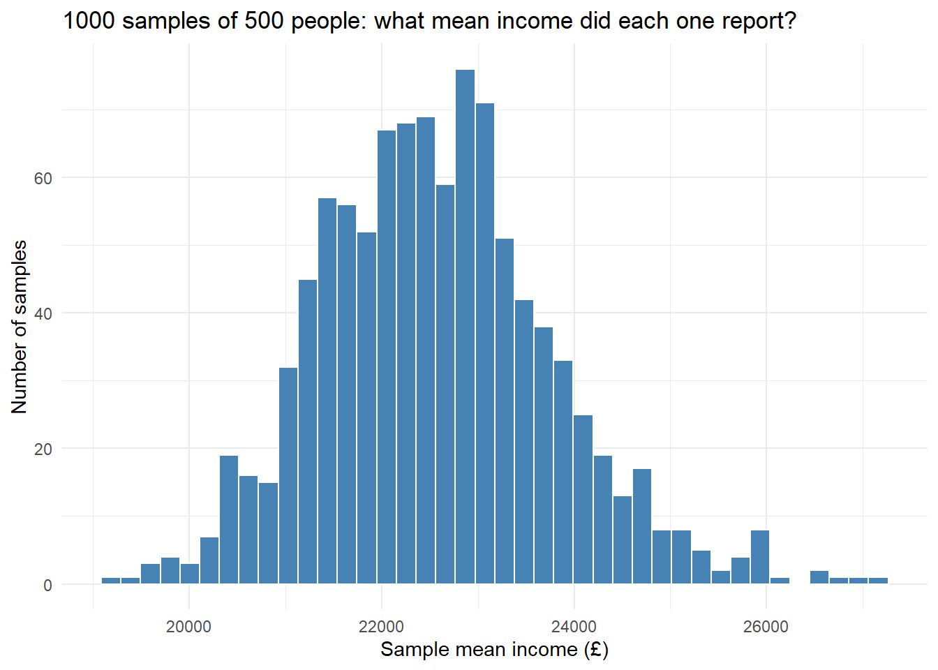
Now let R do it a thousand times and collect all the answers:

many_means <- replicate(1000, mean(sample(frs_independent$income_gross, size = 500)))

replicate(1000, ...) does what its name suggests: it runs whatever is in the brackets 1000 times over and keeps every result. many_means now holds 1000 numbers, each the average income of a different imaginary survey.

means_table <- data.frame(sample_mean = many_means)

ggplot(means_table, aes(x = sample_mean)) +
  geom_histogram(bins = 40, fill = "steelblue", color = "white") +
  labs(
    title = "1000 samples of 500 people: what mean income did each one report?",
    x = "Sample mean income (£)",
    y = "Number of samples"
  ) +
  theme_minimal()

Two things are worth noticing. The histogram is centred on the true value of about £22,500 — samples are not systematically wrong, they are wrong in both directions roughly equally. And it is far narrower than the income distribution you plotted earlier: individual incomes ran from large losses to over a million, but sample means nearly all land within a few thousand pounds of each other.

2.3.2 The Standard Error

The width of that histogram is the thing we want, because it says how far a typical sample lands from the truth. It has a name: the standard error.

sd(many_means)
[1] 1215.977

About £1,200. In other words, a sample of 500 people typically misses the true mean income by around £1,200.

Be careful not to confuse this with the standard deviation of income, which was about £27,000. That one describes how much people differ from each other. The standard error describes how much samples differ from each other. Mixing up the two is one of the most common errors in student reports.

In real life you only ever have one sample, so you cannot build the histogram above. Happily you do not need to — the standard error can be worked out from your single sample, as the standard deviation divided by the square root of the sample size:

sd(frs_independent$income_gross) / sqrt(500)
[1] 1227.262

Compare that with the sd(many_means) value. They agree closely: the formula predicts the width of a histogram we never had to build.

2.3.3 What a P-value Means

From next week onwards, almost every result you produce will come with a p-value attached, so it is worth knowing now what one is.

Suppose we ask whether men and women have different incomes. In our data they clearly do:

frs_independent %>%
  group_by(sex) %>%
  summarise(mean_income = mean(income_gross, na.rm = TRUE), n = n())
# A tibble: 2 × 3
  sex    mean_income     n
  <chr>        <dbl> <int>
1 Female      18134. 17858
2 Male        27473. 15978

A gap of roughly £9,300. But we have just spent half an hour establishing that samples wobble, so before concluding anything about the UK we have to rule out the boring explanation: could a gap this large have turned up purely through the luck of who got sampled, even if men and women earned the same across the country?

That is the question a p-value answers, and it is the only question a p-value answers:

A p-value is: if there were genuinely no difference in the population, how often would sampling alone hand us a gap at least as large as the one we observed?

A small p-value means “hardly ever, so sampling luck is a poor explanation for what I am seeing”. A large p-value means “quite often, so I cannot rule out that this is just noise”. The statement being tested — that there is genuinely no difference in the population — is called the null hypothesis.

t.test(income_gross ~ sex, data = frs_independent)

    Welch Two Sample t-test

data:  income_gross by sex
t = -30.94, df = 26135, p-value < 2.2e-16
alternative hypothesis: true difference in means between group Female and group Male is not equal to 0
95 percent confidence interval:
 -9930.465 -8747.247
sample estimates:
mean in group Female   mean in group Male 
            18134.42             27473.28 

The squiggle ~ is read as “by” or “depends on”, so income_gross ~ sex means “income, broken down by sex”. You will meet this notation constantly from next week, because it is how R writes down a model.

The p-value is reported as < 2.2e-16, R’s way of writing “smaller than 0.00000000000000022”. Sampling variation is essentially impossible as an explanation for a gap this large in a sample this size, so we conclude that a gender income gap exists in the population — not just in our spreadsheet. By convention, a p-value below 0.05 is called statistically significant.

Two warnings to carry into your assignment:

  • A p-value is not the probability that your finding is correct. It is calculated assuming there is no real difference, so it cannot tell you how likely that assumption is.
  • A small p-value does not mean the effect is large or important. With 33,836 people, even a trivial £50 gap would come out “highly significant”. Always report the size of an effect alongside its p-value.

Going further (optional, in your own time): there is more to say about all of this — what a confidence interval really means, why “not significant” does not mean “no difference”, and why Census data needs handling differently. It is written up in Samples, Uncertainty and P-values. You do not need it today, but it will help when you write your report.